Topological World Map

Topology

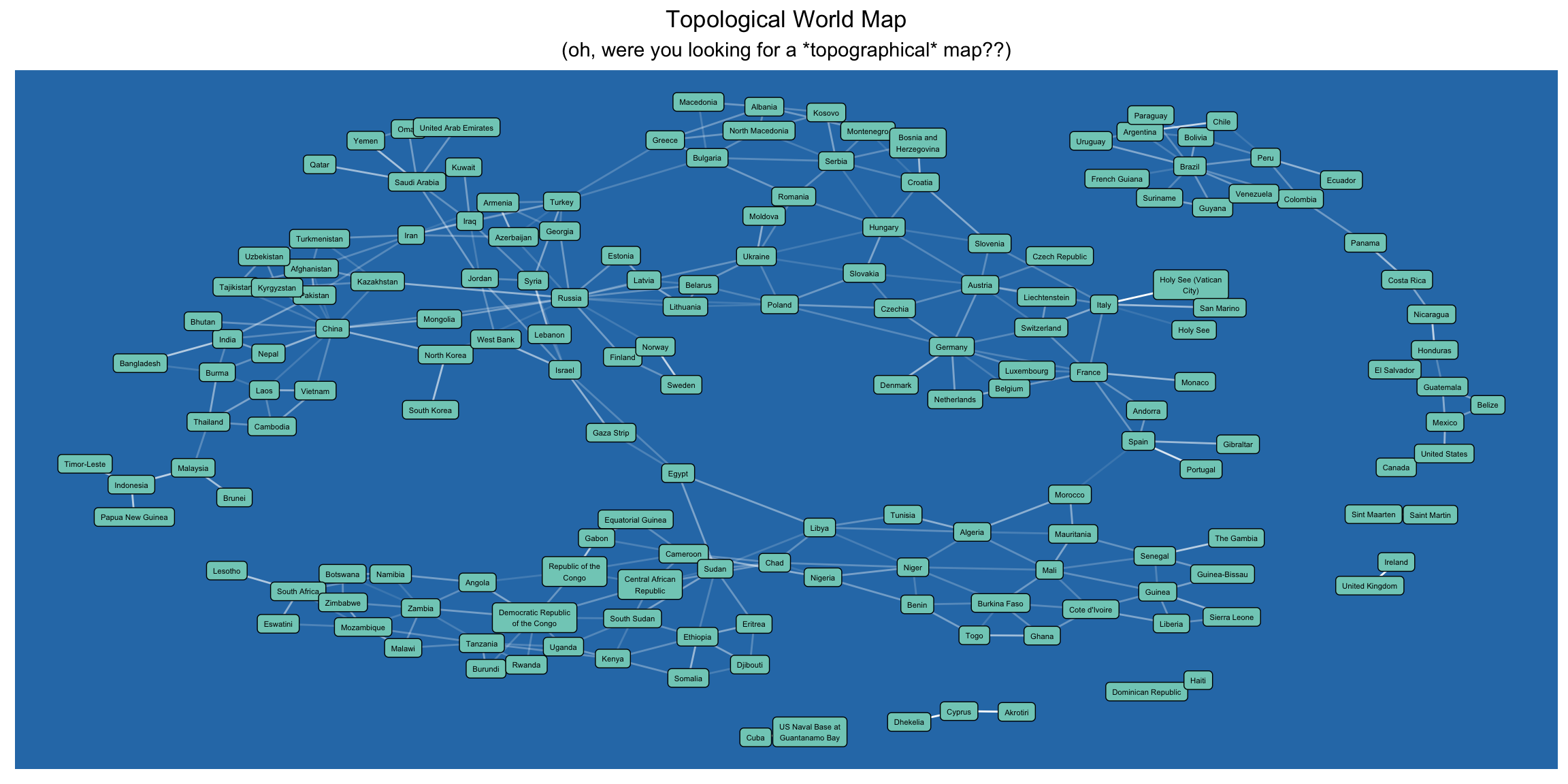
I was looking at the Wikipedia article for topology and noticed that people seemed to get this term confused with topography. As someone who works with networks a lot, I found it a bit funny to think about what a topological map of the world might look like, and how impractical that format of information would be for most practical applications.

So instead of doing any of the thousand things I have on my docket, I of course set out to create such a map (well, technically, graph).

The CIA maintains an online factbook about the world, which includes a list of countries and their land borders/boundaries. We can use rvest to scrape the relevant data from that page.

Code

library(tidyverse)
library(rvest)
library(tidygraph)
library(ggraph)

world_borders <- read_html(
  "https://www.cia.gov/the-world-factbook/field/land-boundaries/"
)

From there, it’s a straightforward (if somewhat tedious) task to extract the relevant pieces of information into a tidy dataframe.

Code

countries <- world_borders %>%
  html_element(".col-lg-9") %>%
  html_element("ul") %>%
  html_elements("li") %>%
  html_text2() %>%
  enframe(name = NULL, value = "source_text") %>%
  mutate(
    # What country are we starting from?
    from = str_remove(source_text, "\n\n[[:print:]\n]*"),
    # From that country, where could we go to?
    to = str_extract(source_text, "\n\n[[:print:]\n]*"),
    to = str_extract(to, "border countries [[:digit:]()]*:\\s.*"),
    to = str_remove(to, "^border countries [[:digit:]()]*:\\s"),
    # What's the total border length of our starting/"from" country?
    total = str_extract(source_text, "total: [[:digit:],\\.]* km"),
    total = str_remove_all(total, "total:|km")
  ) %>%
  # Each bordering country gets its own row
  separate_rows(to, sep = "[;,]\\s") %>%
  mutate(
    # Edge weight is extent of land border
    edge = str_extract(to, "[[:digit:],\\.]* km"),
    edge = str_remove(edge, "\\skm"),
    # Do some cleanup
    from = if_else(from == "Turkey (Turkiye)", "Turkey", from),
    to = str_remove(to, "\\s[[:digit:],\\.]* km"),
    to = str_remove(to, "\\s\\(.*"),
    to = case_when(
      to == "UAE" ~ "United Arab Emirates",
      to == "UK" ~ "United Kingdom",
      to == "US" ~ "United States",
      TRUE ~ to
    ),
    from_pt1 = if_else(
      str_count(from, ",") == 1,
      str_extract(from, "[[:alpha:]]*,"),
      NA_character_
    ),
    from_pt2 = if_else(
      str_count(from, ",") == 1,
      str_extract(from, ", [[:alpha:]\\s]*"),
      NA_character_
    ),
    across(c(from_pt1, from_pt2), ~str_remove(.x, "(\\s,)|,")),
    from = if_else(!is.na(from_pt1), str_c(from_pt2, " ", from_pt1), from)
  ) %>%
  # Fix the column types
  type_convert(
    col_types = cols(from = "c", to = "c", total = "n", edge = "n")
  ) %>%
  # Convert the edge weights from absolute to relative scale
  mutate(edge_standardized = edge / total) %>%
  select(-c(source_text, from_pt1, from_pt2)) %>%
  filter(from != "European Union", from != "World")

We can then use tidygraph to convert this information into a graph representation…

Code

g <- tbl_graph(
  nodes = countries %>%
    drop_na() %>%
    pivot_longer(c(from, to)) %>%
    select(name = value) %>%
    distinct(),
  edges = countries %>%
    drop_na() %>%
    mutate(
      from_sorted = if_else(from < to, from, to),
      to_sorted = if_else(from < to, to, from),
    ) %>%
    arrange(from_sorted, to_sorted) %>%
    group_by(from = from_sorted, to = to_sorted) %>%
    summarise(edge = mean(edge_standardized), .groups = "drop"),
  directed = FALSE
)

And from there, it’s pretty simple to plot it out.

Code

set.seed(sum(utf8ToInt("my angus please stay")))

g %>%
  mutate(name = str_wrap(name, width = 20)) %>%
  ggraph(layout = "fr") +
  geom_edge_fan(
    aes(alpha = edge),
    color = "white",
    show.legend = FALSE
  ) +
  geom_node_label(aes(label = name), size = 1.5, fill = "#80cdc1") +
  ggtitle(
    "Topological World Map",
    subtitle = "(oh, were you looking for a *topographical* map??)"
  ) +
  list(
    theme_bw(),
    theme(
      plot.title = element_text(hjust = 0.5, size = 13),
      plot.subtitle = element_text(hjust = 0.5, size = 11),
      panel.grid.major = element_blank(),
      panel.grid.minor = element_blank(),
      panel.spacing = unit(0.75, "lines"),
      legend.box.spacing = unit(0.5, "lines"),
      legend.margin = margin(c(0, 0, 0, 0), unit = "lines"),
      panel.background = element_rect(fill = "#2c7bb6"),
      panel.border = element_blank(),
      axis.title = element_blank(),
      axis.text = element_blank(),
      axis.ticks = element_blank()
    )
  )